One Country

The smallest complete Posy2 study: one electricity node with demand, onshore wind, and a CCGT. Later examples extend the same pattern of Snapshot, make* builders, optimisation, and result inspection.

using Posy2
using Nosy
using HiGHS
import JuMP: set_silent

# Generate the simulation and configure Posy2 inputs.
sim = Sim(Model(HiGHS.Optimizer); mesh=TimeMesh())
set_silent(model(sim))
example_data_dir = joinpath(pkgdir(Posy2), "data")
snapshot = Snapshot(
    sim,
    Dict(:posy => Posy2Options(
        data_dir=example_data_dir,
        techdata_file="tech_data.xlsx",
        timeseries_file="time_series.xlsx",
        tech_mode=:excel,
        timeseries_mode=:excel,
        discount_rate=0.05,
    )),
)

# Add the electricity and emissions nodes.
# evalprice=true stores electricity node dual prices for reporting.
electricity = Node("country1", EnergyCarrier("electricity country1", sim), rule=:curtailed, evalprice=true, tags=[:electricity])
co2 = Node("CO2", CO2Carrier("CO2", sim), rule=:curtailed, tags=[:co2])

# Hourly electricity demand
makedemand("Demand", "country1", electricity, snapshot)

# Fixed 800 MW wind and continuous CCGT expansion up to 2 GW
makeintermittentsource("Onshore wind", electricity, snapshot; co2_node=co2, tech_column="Onwind", cap=800.0, weather_year=2019)
makedispatchable("CCGT", electricity, snapshot; co2_node=co2, maxcap=2_000.0, unit_size=0.0)

# Minimise total system cost and extract solved values
optimize!(snapshot, cost(snapshot))
result = extract(snapshot)

Expected results:

julia> table(result, capacity)
1×3 DataFrame
 Row │ CCGT country1  Demand country1  Onshore wind country1
     │ Float64        Float64          Float64
─────┼───────────────────────────────────────────────────────
   1 │       889.685              0.0                  800.0

Wind capacity is fixed by the builder at 800 MW. The CCGT capacity is optimised continuously up to maxcap, and the optimiser installs about 890 MW so that residual demand after wind can still be met in every hour.

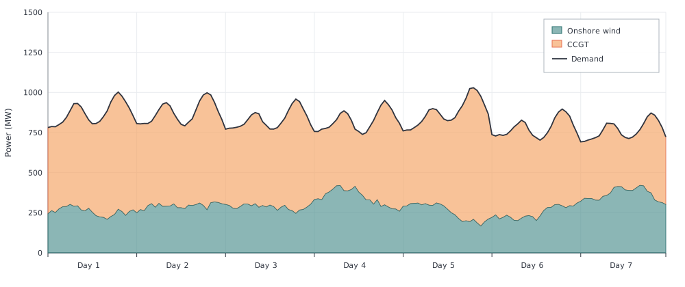
That capacity choice shows up in the hourly dispatch. Over a sample week from the solved year, wind (bottom) and CCGT (top) stack to the black demand line: when wind is strong the CCGT layer shrinks; when wind is weak the CCGT fills the residual, up to the capacity above.

The annual cost breakdown is:

julia> costs(result)[:, [:component, :investment, :fuel, :total]]
4×4 DataFrame
 Row │ component              investment  fuel       total
     │ String                 Float64     Float64    Float64
─────┼─────────────────────────────────────────────────────────
   1 │ CCGT country1           5.80805e7  1.90446e8  2.8712e8
   2 │ Demand country1         0.0        0.0        0.0
   3 │ Onshore wind country1   8.16805e7  0.0        1.14258e8
   4 │ all                     1.39761e8  1.90446e8  4.01378e8

Write the solved result with write_results if you want the workbook report. It returns the path it wrote, and overwrite=true lets the example be re-run over its own output:

julia> write_results(result, "results/one-country.xlsx", overwrite=true)
"results/one-country.xlsx"

That creates results/one-country.xlsx with annual indicators, time series, and price-duration curves. Renaming the node or technology changes which workbook columns Posy2 reads.