Electric Vehicles
The EV API is not fixed yet. The modes, keyword arguments, component and port structure, and reporting semantics may change substantially in later Posy2 versions.
This example compares smart charging and vehicle-to-grid on the same fleet and driving need: how grid charge, discharge, and OCGT generation change.
makeEV picks that behaviour with exactly one of three flags: fixed_profile, smart_charging, or vehicle_to_grid. This page keeps the same demand, PV, OCGT backup, and driving need, and only flips the flag: smart_charging=true first, then vehicle_to_grid=true.
The setup is:
- country1 workbook demand plus an explicit non-uniform daily demand profile
- 1500 MW of PV
- a fleet of 10 000 vehicles
- OCGT backup that covers residual load
Annual net driving (departure − arrival) is fixed by the workbook mobility series and is identical in both runs. With smart charging the optimiser only chooses when to fill the battery. With V2G it also chooses when to sell power back to the node.
Smart charging
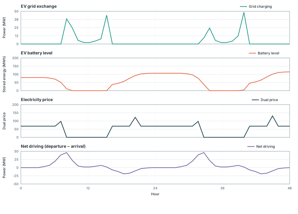
Cars take power from the grid and give it up only as driving. Charge hours are free, so the optimiser charges when the dual is low to cover later driving. With no grid discharge, annual grid charge exceeds annual net driving only by the charging losses: at 90% efficiency, 36 470.80 MWh of charge supports the 32 824 MWh of net driving.
using Posy2
using Nosy
using HiGHS
import JuMP: set_silent

# Simulation and Posy2 input configuration
sim = Sim(Model(HiGHS.Optimizer); mesh=TimeMesh())
set_silent(model(sim))
example_data_dir = joinpath(pkgdir(Posy2), "data")
snapshot = Snapshot(sim, Dict(:posy => Posy2Options(
    data_dir=example_data_dir,
    techdata_file="tech_data.xlsx",
    timeseries_file="time_series.xlsx",
    tech_mode=:arguments,
    timeseries_mode=:excel,
)))

# Electricity node (evalprice for dualprice) and CO2 sink
electricity = Node("country1", EnergyCarrier("electricity country1", sim), rule=:curtailed, evalprice=true, tags=[:electricity])
co2 = Node("CO2", CO2Carrier("CO2", sim), rule=:curtailed, tags=[:co2])

# Hourly electricity demand from the time-series workbook
makedemand("Demand", "country1", electricity, snapshot)

# Additional exogenous demand with distinct morning and evening peaks
daily_extra_demand = Float64[
    30, 15, 0, 0, 15, 45, 90, 140, 80, 30, 0, 40,
    110, 50, 10, 20, 70, 150, 100, 30, 90, 60, 30, 20,
]
makedemand(
    "Variable demand", "country1", electricity, snapshot;
    profile=repeat(daily_extra_demand, 365),
)

# Fixed 1500 MW PV
makeintermittentsource(
    "Solar", electricity, snapshot; co2_node=co2, tech_column="PV",
    cap=1500.0,
    weather_year=2019,
)

# Smart-charging fleet: 10 000 vehicles; charge only
makeEV(
    "EV", electricity, snapshot;
    number_ev=10000.0,                 # vehicles
    initial_connected_share=1.0,
    fixed_profile=false,
    smart_charging=true,
    zone="country1",
    charging_eff=0.9,
    max_charging_power_per_ev=0.01,     # MW per vehicle, * fleet size
    battery_capacity_per_ev=0.06,       # MWh per vehicle, * fleet size
)

# Fixed OCGT backup (continuous UC with startup cost, same plant in both cases)
makedispatchable(
    "OCGT", electricity, snapshot; co2_node=co2, tech_column="OCGT",
    cap=1200.0,
    fuel_cost=68.24,
    unit_size=100.0,
    uc=true,
    startup_cost=6_270.0,
    min_power=0.3,
    min_uptime=2.0,
    min_downtime=2.0,
    startup_duration=1.0,
    shutdown_duration=1.0,
)

# Minimise total system cost and extract solved values
optimize!(snapshot, cost(snapshot))
result = extract(snapshot)
Annual net driving is 32 824 MWh. Charge is higher because of the 90% charging efficiency, and nothing is sold to the node. OCGT still covers residual demand:
julia> driving = balance(result, "EV country1", :output, energy; collapse=true, aggregate=false)["driving"]
32823.71999999754

julia> charge = balance(result, "EV country1", :input, energy; collapse=true, aggregate=false)["input"]
36470.79999999986

julia> balance(result, "OCGT country1", :output, energy; collapse=true, aggregate=true)
5.098481783239689e6
The figure uses 25–26 June, when the additional demand peaks, PV, and OCGT commitment produce several price levels. Charging lines up with lower duals, and the battery-level panel shows how energy moves between charging and the driving series. Nothing is sold back to the node.
Vehicle-to-grid
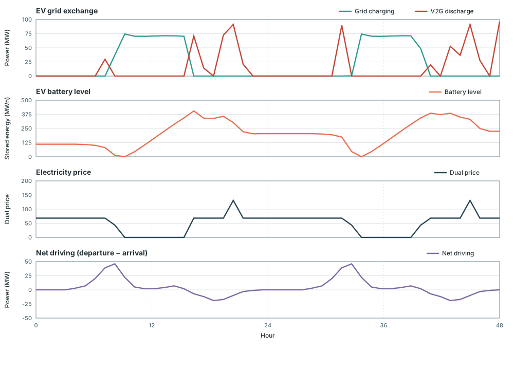
The same fleet keeps the same departure and arrival series, and may also inject into the electricity node. Discharge adds a compensation cost per MWh, so the optimiser sells back mainly when the node dual is high enough to cover that cost. Charging gathers when the dual is low.
using Posy2
using Nosy
using HiGHS
import JuMP: set_silent

# Simulation and Posy2 input configuration
sim = Sim(Model(HiGHS.Optimizer); mesh=TimeMesh())
set_silent(model(sim))
example_data_dir = joinpath(pkgdir(Posy2), "data")
snapshot = Snapshot(sim, Dict(:posy => Posy2Options(
    data_dir=example_data_dir,
    techdata_file="tech_data.xlsx",
    timeseries_file="time_series.xlsx",
    tech_mode=:arguments,
    timeseries_mode=:excel,
)))

# Electricity node (evalprice for dualprice) and CO2 sink
electricity = Node("country1", EnergyCarrier("electricity country1", sim), rule=:curtailed, evalprice=true, tags=[:electricity])
co2 = Node("CO2", CO2Carrier("CO2", sim), rule=:curtailed, tags=[:co2])

# Hourly electricity demand from the time-series workbook
makedemand("Demand", "country1", electricity, snapshot)

# Same additional exogenous demand as in the smart-charging case
daily_extra_demand = Float64[
    30, 15, 0, 0, 15, 45, 90, 140, 80, 30, 0, 40,
    110, 50, 10, 20, 70, 150, 100, 30, 90, 60, 30, 20,
]
makedemand(
    "Variable demand", "country1", electricity, snapshot;
    profile=repeat(daily_extra_demand, 365),
)

# Fixed 1500 MW PV (same as smart-charging case)
makeintermittentsource(
    "Solar", electricity, snapshot; co2_node=co2, tech_column="PV",
    cap=1500.0,
    weather_year=2019,
)

# Same fleet as smart charging, with grid discharge enabled
makeEV(
    "EV", electricity, snapshot;
    number_ev=10000.0,                 # same fleet as smart charging
    initial_connected_share=1.0,
    fixed_profile=false,
    vehicle_to_grid=true,
    zone="country1",
    charging_eff=0.9,
    max_charging_power_per_ev=0.01,     # MW per vehicle, * fleet size
    max_dispatch_power_per_ev=0.01,     # MW per vehicle V2G rating, * fleet size
    battery_capacity_per_ev=0.06,       # MWh per vehicle, * fleet size
    compensation=20.0,                  # currency/MWh on grid discharge
)

# Same OCGT plant as the smart-charging case
makedispatchable(
    "OCGT", electricity, snapshot; co2_node=co2, tech_column="OCGT",
    cap=1200.0,
    fuel_cost=68.24,
    unit_size=100.0,
    uc=true,
    startup_cost=6_270.0,
    min_power=0.3,
    min_uptime=2.0,
    min_downtime=2.0,
    startup_duration=1.0,
    shutdown_duration=1.0,
)

# Minimise total system cost and extract solved values
optimize!(snapshot, cost(snapshot))
result = extract(snapshot)
Driving stays at 32 824 MWh. With V2G the fleet can also sell power back, so it cycles like a battery: annual charge rises well above driving, grid discharge appears, and OCGT generation reduces:
julia> driving = balance(result, "EV country1", :output, energy; collapse=true, aggregate=false)["driving"]
32823.71999999754

julia> discharge = balance(result, "EV country1", :output, energy; collapse=true, aggregate=false)["output"]
57748.54945157862

julia> charge = balance(result, "EV country1", :input, energy; collapse=true, aggregate=false)["input"]
100635.85494619841

julia> balance(result, "OCGT country1", :output, energy; collapse=true, aggregate=true)
5.056856913300684e6

julia> price = dualprice(result.nodes["country1"]);

julia> sort(unique(round.(price[4201:4248]; digits=3)))
4-element Vector{Float64}:
   0.0
  43.416
  68.24
 130.94
dualprice returns the hourly node dual. The selected two-day window contains four price levels rather than the nearly flat winter window.
On the same June window as above, charge sits under low duals and V2G discharge appears under higher duals. The battery-level curve makes the intertemporal balance visible when discharge and charging differ within the plotted window.
Comparing the two modes
Both runs keep the same country1 demand, 1500 MW of PV, OCGT backup, and 10 000 vehicles. Only the EV mode flag flips from smart_charging=true to vehicle_to_grid=true. Smart charging exposes departure, arrival, and reporting driving. V2G adds a grid output (discharge). Driving energy matches in both cases. OCGT generation reduces under V2G because that discharge can cover residual load.
| Smart | V2G | |
|---|---|---|
:output / :input ports | departure, driving / arrival | departure, driving, output / arrival |
| Grid discharge (MWh/year) | 0 | 57749 |
| OCGT generation (MWh/year) | 5.098e6 | 5.057e6 |
| Driving energy (MWh/year) | 32824 | 32824 |